4.3. Manipulating brain volume: input/output, masking, ROIs, smoothing...

This chapter presents the structure of brain image data and tools to manipulation them.

4.3.1. Loading data

4.3.1.1. Fetching datasets

Nilearn package embeds a dataset fetching utility to download reference datasets and atlases. Dataset fetching functions can be imported from nilearn.datasets:

>>> from nilearn import datasets
>>> haxby_files = datasets.fetch_haxby(n_subjects=1)

They return a structure that contains the different file names:

>>> # The different files
>>> print(list(haxby_files.keys()))
['mask_house_little', 'anat', 'mask_house', 'mask_face', 'func', 'session_target', 'mask_vt', 'mask_face_little']
>>> # Path to first functional file
>>> print(haxby_files.func[0])  
/.../nilearn_data/haxby2001/subj1/bold.nii.gz
>>> # Provide information on the dataset
>>> print(haxby_files.description) 
Haxby 2001 results


Notes
-----
Results from a classical fMRI study that...

An explanations and further resources about the dataset at hand can be retrieved as follows:

>>> print haxby_dataset['description']

For a list of all the data fetching functions in nilearn, see nilearn.datasets: Automatic Dataset Fetching.

The data are downloaded only once and stored locally, in one of the following directories (in order of priority):

• default system paths used by third party softwares that may already have downloaded of could benefit of this data
• the folder specified by data_dir parameter in the fetching function if it is specified
• the global environment variable NILEARN_SHARED_DATA if it exists
• the user environment variable NILEARN_DATA if it exists
• the nilearn_data folder in the user home folder

Two different environment variables are provided to distinguish a global dataset repository that may be read-only from a user-level one. Note that you can copy that folder across computers to avoid downloading the data twice.

4.3.1.2. Loading your own data

Using your own experiment in nilearn is as simple as declaring a list of your files

# dataset folder contains subject1.nii and subject2.nii
my_data = ['dataset/subject1.nii', 'dataset/subject2.nii']

Python also provides helpers to work with filepaths. In particular, glob.glob is useful to list many files with a “wild-card”: *.nii

Warning

The result of glob.glob is not sorted. For neuroimaging, you should always sort the output of glob using the sorted function.

>>> # dataset folder contains subject1.nii and subject2.nii
>>> import glob
>>> sorted(glob.glob('dataset/subject*.nii')) 
['dataset/subject1.nii', 'dataset/subject2.nii']

4.3.2. Understanding Neuroimaging data

4.3.2.1. Nifti and Analyze files

NIfTI and Analyze file structures

NifTi files (or Analyze files) are the standard way of sharing data in neuroimaging. We may be interested in the following three main components:

data:raw scans bundled in a numpy array: data = img.get_data() affine:gives the correspondance between voxel index and spatial location: affine = img.get_affine() header:informations about the data (slice duration...): header = img.get_header()

Neuroimaging data can be loaded simply thanks to nibabel. Once the file is downloaded, a single line is needed to load it.

Dataset formatting: data shape

We can find two main representations for MRI scans:

• a big 4D matrix representing 3D MRI along time, stored in a big 4D NifTi file. FSL users tend to prefer this format.
• several 3D matrices representing each volume (time point) of the session, stored in set of 3D Nifti or analyse files. SPM users tend to prefer this format.

4.3.2.2. Niimg-like objects

Often, nilearn functions take as input parameters what we call “Niimg-like objects:

Niimg: A Niimg-like object can either be:

• a file path to a Nifti or Analyse image
• any object exposing get_data() and get_affine() methods, for instance a Nifti1Image from nibabel.

Niimg-4D: Similarly, some functions require 4-dimensional Nifti-like data, which we call Niimgs, or Niimg-4D. Accepted inputs are then:

• A path to a 4-dimensional Nifti image
• List of paths to 3-dimensional Nifti images
• 4-dimensional Nifti-like object
• List of 3-dimensional Nifti-like objects

Note

Image affines

If you provide a sequence of Nifti images, all of them must have the same affine.

4.3.2.3. Text files: phenotype or behavior

Phenotypic or behavioral data are often provided as text or CSV (Comma Separated Values) file. They can be loaded with numpy.genfromtxt but you may have to specify some options (typically skip_header ignores column titles if needed).

For the Haxby datasets, we can load the categories of the images presented to the subject:

>>> from nilearn import datasets
>>> haxby_dataset = datasets.fetch_haxby(n_subjects=1)
>>> import numpy as np
>>> labels = np.recfromcsv(haxby_dataset.session_target[0], delimiter=" ")
>>> stimuli = labels['labels']
>>> print(np.unique(stimuli))
['bottle' 'cat' 'chair' 'face' 'house' 'rest' 'scissors' 'scrambledpix'
 'shoe']

4.3.3. Masking data manually

4.3.3.1. Extracting a brain mask

If we do not have a mask of the relevant regions available, a brain mask can be easily extracted from the fMRI data using the nilearn.masking.compute_epi_mask function:

compute_epi_mask(epi_img[, lower_cutoff, ...])

Compute a brain mask from fMRI data in 3D or 4D ndarrays.

# Simple computation of a mask from the fMRI data
from nilearn.masking import compute_epi_mask
mask_img = compute_epi_mask(func_filename)

plot_roi(mask_img, mean_haxby)

4.3.3.2. From 4D to 2D arrays

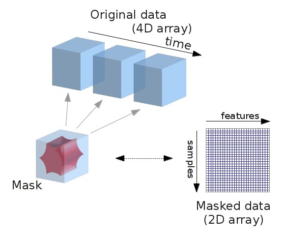
fMRI data is usually represented as a 4D block of data: 3 spatial dimensions and one of time. In practice, we are most often only interested in working only on the time-series of the voxels in the brain. It is thus convenient to apply a brain mask and go from a 4D array to a 2D array, voxel x time, as depicted below:

from nilearn.masking import apply_mask
masked_data = apply_mask(func_filename, mask_img)

# masked_data shape is (timepoints, voxels). We can plot the first 150
# timepoints from two voxels

plt.figure(figsize=(7, 5))
plt.plot(masked_data[:2, :150].T)
plt.xlabel('Time [TRs]', fontsize=16)
plt.ylabel('Intensity', fontsize=16)
plt.xlim(0, 150)
plt.subplots_adjust(bottom=.12, top=.95, right=.95, left=.12)

plt.show()

4.3.4. Functions for data preparation steps

The NiftiMasker automatically does some important data preparation steps. These steps are also available as simple functions if you want to set up your own data preparation procedure:

• Resampling: nilearn.image.resample_img. See the example example_manipulating_visualizing_plot_affine_transformation.py to see the effect of affine transforms on data and bounding boxes.
• Computing the mean of images (in the time of 4th direction): nilearn.image.mean_img
• Swapping voxels of both hemisphere: nilearn.image.swap_img_hemispheres
• Smoothing: nilearn.image.smooth_img
• Masking:
  • compute from EPI images: nilearn.masking.compute_epi_mask
  • compute from images with a flat background: nilearn.masking.compute_background_mask
  • compute for multiple sessions/subjects: nilearn.masking.compute_multi_epi_mask nilearn.masking.compute_multi_background_mask
  • apply: nilearn.masking.apply_mask
  • intersect several masks (useful for multi sessions/subjects): nilearn.masking.intersect_masks
  • unmasking: nilearn.masking.unmask
• Cleaning signals: nilearn.signal.clean

4.3.5. Image operations: creating a ROI mask manually

This section shows manual steps to create and finally control an ROI mask. They are a good example of using basic image manipulation on Nifti images.

4.3.5.1. Smoothing

Functional MRI data has a low signal-to-noise ratio. When using simple methods that are not robust to noise, it is useful to smooth the data. Smoothing is usually applied using a Gaussian function with 4mm to 8mm full-width at half-maximum. The function nilearn.image.smooth_img accounts for potential anisotropy in the image affine. As many nilearn functions, it can also use file names as input parameters.

from nilearn import image
fmri_filename = haxby_dataset.func[0]
fmri_img = image.smooth_img(fmri_filename, fwhm=6)

# Plot the mean image
mean_img = image.mean_img(fmri_img)
plot_epi(mean_img, title='Smoothed mean EPI', cut_coords=cut_coords)

4.3.5.2. Selecting features

Functional MRI data are high dimensional compared to the number of samples (usually 50000 voxels for 1000 samples). In this setting, machine learning algorithm can perform poorly. However, a simple statistical test can help reducing the number of voxels.

The Student’s t-test (scipy.stats.ttest_ind) performs a simple statistical test that determines if two distributions are statistically different. It can be used to compare voxel timeseries in two different conditions (when houses or faces are shown in our case). If the timeserie distribution is similar in the two conditions, then the voxel is not very interesting to discriminate the condition.

This test returns p-values that represents probabilities that the two timeseries are drawn from the same distribution. The lower is the p-value, the more discriminative is the voxel.

from scipy import stats
fmri_data = fmri_img.get_data()
_, p_values = stats.ttest_ind(fmri_data[..., haxby_labels == b'face'],
                              fmri_data[..., haxby_labels == b'house'],
                              axis=-1)

# Use a log scale for p-values
log_p_values = -np.log10(p_values)
log_p_values[np.isnan(log_p_values)] = 0.
log_p_values[log_p_values > 10.] = 10.
plot_stat_map(new_img_like(fmri_img, log_p_values),
              mean_img, title="p-values", cut_coords=cut_coords)

This feature selection method is available in the scikit-learn where it has been extended to several classes, using the sklearn.feature_selection.f_classif function.

4.3.5.3. Thresholding

Higher p-values are kept as voxels of interest. Applying a threshold to an array is easy thanks to numpy indexing a la Matlab.

log_p_values[log_p_values < 5] = 0
plot_stat_map(new_img_like(fmri_img, log_p_values),
              mean_img, title='Thresholded p-values', annotate=False,
              colorbar=False, cut_coords=cut_coords)

4.3.5.4. Mask intersection

We now want to restrict our study to the ventral temporal area. The corresponding mask is provided in haxby.mask_vt. We want to compute the intersection of this mask with our mask. The first step is to load it with nibabel’s nibabel.load. We then use a logical “and” – numpy.logical_and – to keep only voxels that are selected in both masks.

# (intersection corresponds to an "AND conjunction")
bin_p_values = (log_p_values != 0)
mask_vt_filename = haxby_dataset.mask_vt[0]
vt = nibabel.load(mask_vt_filename).get_data().astype(bool)
bin_p_values_and_vt = np.logical_and(bin_p_values, vt)

plot_roi(new_img_like(fmri_img, bin_p_values_and_vt.astype(np.int)),
         mean_img, title='Intersection with ventral temporal mask',
         cut_coords=cut_coords)

4.3.5.5. Mask dilation

We observe that our voxels are a bit scattered across the brain. To obtain more compact shape, we use a morphological dilation. This is a common step to be sure not to forget voxels located on the edge of a ROI.

from scipy import ndimage
dil_bin_p_values_and_vt = ndimage.binary_dilation(bin_p_values_and_vt)
plot_roi(new_img_like(fmri_img, dil_bin_p_values_and_vt.astype(np.int)),
         mean_img, title='Dilated mask', cut_coords=cut_coords,
         annotate=False)

4.3.5.6. Extracting connected components

Scipy function scipy.ndimage.label identifies connected components in our final mask: it assigns a separate integer label to each one of them.

plt.figure()
labels, n_labels = ndimage.label(dil_bin_p_values_and_vt)
first_roi_data = (labels == 1).astype(np.int)
second_roi_data = (labels == 2).astype(np.int)
fig_id = plt.subplot(2, 1, 1)
plot_roi(new_img_like(fmri_img, first_roi_data),
         mean_img, title='Connected components: first ROI', axes=fig_id)
fig_id = plt.subplot(2, 1, 2)
plot_roi(new_img_like(fmri_img, second_roi_data),
         mean_img, title='Connected components: second ROI', axes=fig_id)
plt.subplots_adjust(left=0, right=1, bottom=0, top=1, hspace=0)
plot_roi(new_img_like(fmri_img, first_roi_data),
         mean_img, title='Connected components: first ROI_',
         output_file='snapshot_first_ROI.png')
plot_roi(new_img_like(fmri_img, second_roi_data),
         mean_img, title='Connected components: second ROI',
         output_file='snapshot_second_ROI.png')

4.3.5.7. Saving the result

The final result is saved using nibabel for further consultation with a software like FSLview for example.

nibabel.save(new_img_like(fmri_img, labels),
             'mask_atlas.nii')