2.1. A decoding tutorial
This page is a decoding tutorial articulated on the analysis of the Haxby 2001 dataset. It shows how to predict from brain activity images the stimuli that the subject is viewing.
Contents
2.1.1. Data loading and preparation
2.1.1.1. The Haxby 2001 experiment
Subjects are presented visual stimuli from different categories. We are going to predict which category the subject is seeing from the fMRI activity recorded in masks of the ventral stream. Significant prediction shows that the signal in the region contains information on the corresponding category.
2.1.1.2. Loading the data into Python
Launch IPython:
ipython --matplotlib
First, load the data using nilearn data downloading function,
nilearn.datasets.fetch_haxby:
from nilearn import datasets
haxby_dataset = datasets.fetch_haxby()

# print basic information on the dataset
print('First subject anatomical nifti image (3D) is at: %s' %
      haxby_dataset.anat[0])
print('First subject functional nifti images (4D) are at: %s' %
      haxby_dataset.func[0])  # 4D data
The haxby_dataset object has several entries that contain paths to the files
downloaded on the disk:
>>> print(haxby_dataset)
{'anat': ['/home/varoquau/dev/nilearn/nilearn_data/haxby2001/subj1/anat.nii.gz'],
'func': ['/home/varoquau/dev/nilearn/nilearn_data/haxby2001/subj1/bold.nii.gz'],
'mask_face': ['/home/varoquau/dev/nilearn/nilearn_data/haxby2001/subj1/mask8b_face_vt.nii.gz'],
'mask_face_little': ['/home/varoquau/dev/nilearn/nilearn_data/haxby2001/subj1/mask8_face_vt.nii.gz'],
'mask_house': ['/home/varoquau/dev/nilearn/nilearn_data/haxby2001/subj1/mask8b_house_vt.nii.gz'],
'mask_house_little': ['/home/varoquau/dev/nilearn/nilearn_data/haxby2001/subj1/mask8_house_vt.nii.gz'],
'mask_vt': ['/home/varoquau/dev/nilearn/nilearn_data/haxby2001/subj1/mask4_vt.nii.gz'],
'session_target': ['/home/varoquau/dev/nilearn/nilearn_data/haxby2001/subj1/labels.txt']}
We load the behavioral labels from the corresponding text file and limit our analysis to the face and cat conditions:
import numpy as np
# Load target information as string and give a numerical identifier to each
labels = np.recfromcsv(haxby_dataset.session_target[0], delimiter=" ")

# scikit-learn >= 0.14 supports text labels. You can replace this line by:
# target = labels['labels']
_, target = np.unique(labels['labels'], return_inverse=True)

### Keep only data corresponding to faces or cats #############################
condition_mask = np.logical_or(labels['labels'] == b'face',
                               labels['labels'] == b'cat')
target = target[condition_mask]
Then we prepare the fMRI data: we use the NiftiMasker to apply the
mask_vt mask to the 4D fMRI data, so that its shape becomes (n_samples,
n_features) (see From 4D to 2D arrays for a discussion on using masks).
Note
seemingly minor data preparation can matter a lot on the final score, for instance standardizing the data.
from nilearn.input_data import NiftiMasker
mask_filename = haxby_dataset.mask_vt[0]
# For decoding, standardizing is often very important
nifti_masker = NiftiMasker(mask_img=mask_filename, standardize=True)

func_filename = haxby_dataset.func[0]
# We give the nifti_masker a filename and retrieve a 2D array ready
# for machine learning with scikit-learn
fmri_masked = nifti_masker.fit_transform(func_filename)

# Restrict the classification to the face vs cat discrimination
fmri_masked = fmri_masked[condition_mask]
2.1.2. Performing the decoding analysis
2.1.2.1. The prediction engine
2.1.2.1.1. An estimator object
To perform decoding we construct an estimator, predicting a condition label y given a set X of images.
We use here a simple Support Vector Classification (or SVC) with a
linear kernel. We first import the correct module from scikit-learn and we
define the classifier, sklearn.svm.SVC:
from sklearn.svm import SVC
svc = SVC(kernel='linear')
The documentation of the object details all parameters. In IPython, it can be displayed as follows:
In [10]: svc?
Type:             SVC
Base Class:       <class 'sklearn.svm.libsvm.SVC'>
String Form:
SVC(kernel=linear, C=1.0, probability=False, degree=3, coef0=0.0, eps=0.001,
cache_size=100.0, shrinking=True, gamma=0.0)
Namespace:        Interactive
Docstring:
    C-Support Vector Classification.
    Parameters
    ----------
    C : float, optional (default=1.0)
        penalty parameter C of the error term.
...
See also
2.1.2.1.2. Applying it to data: fit (train) and predict (test)
In scikit-learn, the prediction objects have two important methods:
- a fit function that “learns” the parameters of the model from the data. Thus, we need to give some training data to fit.
- a predict function that “predicts” a target from new data. Here, we just have to give the new set of images (as the target should be unknown):
svc.fit(fmri_masked, target)
prediction = svc.predict(fmri_masked)
Warning
Do not predict on data used by the fit: the prediction that we obtain here is to good to be true (see next paragraph). Here we are just doing a sanity check.
2.1.2.2. Measuring prediction performance
2.1.2.2.1. Cross-validation
However, the last analysis is wrong, as we have learned and tested on the same set of data. We need to use a cross-validation to split the data into different sets, called “folds”, in a K-Fold strategy.
We use a cross-validation object,
sklearn.cross_validation.KFold, that simply generates the
indices of the folds within a loop.
from sklearn.cross_validation import KFold

cv = KFold(n=len(fmri_masked), n_folds=5)
cv_scores = []

for train, test in cv:
    svc.fit(fmri_masked[train], target[train])
    prediction = svc.predict(fmri_masked[test])
    cv_scores.append(np.sum(prediction == target[test])
                     / float(np.size(target[test])))

print(cv_scores)
There is a specific function,
sklearn.cross_validation.cross_val_score that computes for you
the score for the different folds of cross-validation:
>>> from sklearn.cross_validation import cross_val_score
>>> cv_scores = cross_val_score(svc, fmri_masked, target, cv=cv)
You can speed up the computation by using n_jobs=-1, which will spread the computation equally across all processors (but will probably not work under Windows):
>>> cv_scores = cross_val_score(svc, fmri_masked, target, cv=cv, n_jobs=-1, verbose=10)
Prediction accuracy: We can take a look at the results of the cross_val_score function:
>>> print(cv_scores)
[0.72727272727272729, 0.46511627906976744, 0.72093023255813948, 0.58139534883720934, 0.7441860465116279]
This is simply the prediction score for each fold, i.e. the fraction of correct predictions on the left-out data.
2.1.2.2.2. Choosing a good cross-validation strategy
There are many cross-validation strategies possible, including K-Fold or leave-one-out. When choosing a strategy, keep in mind that:
- The test set should be as litte correlated as possible with the train set
- The test set needs to have enough samples to enable a good measure of the prediction error (a rule of thumb is to use 10 to 20% of the data).
In these regards, leave one out is often one of the worst options.
Here, in the Haxby example, we are going to leave a session out, in order
to have a test set independent from the train set. For this, we are going
to use the session label, present in the behavioral data file, and
sklearn.cross_validation.LeaveOneLabelOut:
>>> from sklearn.cross_validation import LeaveOneLabelOut
>>> session_label = labels['chunks']
>>> # We need to remember to remove the rest conditions
>>> session_label = session_label[condition_mask]
>>> cv = LeaveOneLabelOut(labels=session_label)
>>> cv_scores = cross_val_score(svc, fmri_masked, target, cv=cv)
>>> print(cv_scores)
[ 1.          0.61111111  0.94444444  0.88888889  0.88888889  0.94444444
  0.72222222  0.94444444  0.5         0.72222222  0.5         0.55555556]
Exercise
Compute the mean prediction accuracy using cv_scores
Solution
>>> classification_accuracy = np.mean(cv_scores)
>>> classification_accuracy
0.76851851851851849
We have a total prediction accuracy of 77% across the different sessions.
2.1.2.2.3. Choice of the prediction accuracy measure
The default metric used for measuring errors is the accuracy score, i.e. the number of total errors. It is not always a sensible metric, especially in the case of very imbalanced classes, as in such situations choosing the dominant class can achieve a low number of errors.
Other metrics, such as the f1-score, can be used:
>>> cv_scores = cross_val_score(svc, fmri_masked, target, cv=cv, scoring='f1')
See also
2.1.2.2.4. Measuring the chance level
Dummy estimators: The simplest way to measure prediction performance
at chance, is to use a dummy classifier,
sklearn.dummy.DummyClassifier:
>>> from sklearn.dummy import DummyClassifier
>>> null_cv_scores = cross_val_score(DummyClassifier(), fmri_masked, target, cv=cv)
Permutation testing: A more controlled way, but slower, is to do
permutation testing on the labels, with
sklearn.cross_validation.permutation_test_score:
>>> from sklearn.cross_validation import permutation_test_score
>>> null_cv_scores = permutation_test_score(svc, fmri_masked, target, cv=cv)
Putting it all together
The ROI-based decoding example does a decoding analysis per mask, giving the f1-score of the prediction for each object.
It uses all the notions presented above, with for loop to iterate
over masks and categories and Python dictionnaries to store the
scores.
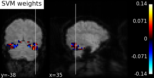
2.1.2.3. Visualizing the decoder’s weights
We can visualize the weights of the decoder:
- we first inverse the masking operation, to retrieve a 3D brain volume of the SVC’s weights.
- we then create a figure and plot as a background the first EPI image
- finally we plot the SVC’s weights after masking the zero values
# Retrieve the SVC discriminating weights
coef_ = svc.coef_

# Reverse masking thanks to the Nifti Masker
coef_img = nifti_masker.inverse_transform(coef_)

# Save the coefficients as a Nifti image
coef_img.to_filename('haxby_svc_weights.nii')

### Visualization #############################################################
import matplotlib.pyplot as plt
from nilearn.image.image import mean_img
from nilearn.plotting import plot_roi, plot_stat_map

mean_epi = mean_img(func_filename)
plot_stat_map(coef_img, mean_epi, title="SVM weights", display_mode="yx")

plot_roi(nifti_masker.mask_img_, mean_epi, title="Mask", display_mode="yx")

plt.show()
See also
2.1.3. Decoding without a mask: Anova-SVM
2.1.3.1. Dimension reduction with feature selection
If we do not start from a mask of the relevant regions, there is a very large number of voxels and not all are useful for face vs cat prediction. We thus add a feature selection procedure. The idea is to select the k voxels most correlated to the task.
For this, we need to import the sklearn.feature_selection module and use
sklearn.feature_selection.f_classif, a simple F-score
based feature selection (a.k.a.
Anova),
that we will put before the SVC in a pipeline
(sklearn.pipeline.Pipeline):
from sklearn.feature_selection import SelectKBest, f_classif

### Define the dimension reduction to be used.
# Here we use a classical univariate feature selection based on F-test,
# namely Anova. We set the number of features to be selected to 500
feature_selection = SelectKBest(f_classif, k=500)

# We have our classifier (SVC), our feature selection (SelectKBest), and now,
# we can plug them together in a *pipeline* that performs the two operations
# successively:
from sklearn.pipeline import Pipeline
anova_svc = Pipeline([('anova', feature_selection), ('svc', svc)])

### Fit and predict ###########################################################

anova_svc.fit(X, y)
y_pred = anova_svc.predict(X)
We can use our anova_svc object exactly as we were using our svc
object previously.
2.1.3.2. Visualizing the results
To visualize the results, we need to:
- first get the support vectors of the SVC and inverse the feature selection mechanism
- then, as before, inverse the masking process to retrieve the weights and plot them.
### Look at the SVC's discriminating weights
coef = svc.coef_
# reverse feature selection
coef = feature_selection.inverse_transform(coef)
# reverse masking
weight_img = nifti_masker.inverse_transform(coef)


### Create the figure
from nilearn import image
import matplotlib.pyplot as plt
from nilearn.plotting import plot_stat_map

# Plot the mean image because we have no anatomic data
mean_img = image.mean_img(func_filename)

plot_stat_map(weight_img, mean_img, title='SVM weights')

### Saving the results as a Nifti file may also be important
weight_img.to_filename('haxby_face_vs_house.nii')
See also
Final script
The complete script to do an SVM-Anova analysis can be found as an example.
2.1.4. Going further with scikit-learn
We have seen a very simple analysis with scikit-learn, but it may be interesting to explore the wide variety of supervised learning algorithms in the scikit-learn.
2.1.4.1. Changing the prediction engine
We now see how one can easily change the prediction engine, if needed. We can try Fisher’s Linear Discriminant Analysis (LDA)
Import the module:
>>> from sklearn.lda import LDA
Construct the new estimator object and use it in a pipeline:
>>> from sklearn.pipeline import Pipeline
>>> lda = LDA()
>>> anova_lda = Pipeline([('anova', feature_selection), ('LDA', lda)])
and recompute the cross-validation score:
>>> cv_scores = cross_val_score(anova_lda, X, y, cv=cv, verbose=1)
>>> classification_accuracy = np.mean(cv_scores)
>>> print("Classification accuracy: %.4f / Chance Level: %.4f" % \
...    (classification_accuracy, 1. / n_conditions))
Classification accuracy: 1.0000 / Chance level: 0.5000
2.1.4.2. Changing the feature selection
Let’s say that you want a more sophisticated feature selection, for example a Recursive Feature Elimination (RFE)
Import the module:
>>> from sklearn.feature_selection import RFE
Construct your new fancy selection:
>>> rfe = RFE(SVC(kernel='linear', C=1.), 50, step=0.25)
and create a new pipeline:
>>> rfe_svc = Pipeline([('rfe', rfe), ('svc', clf)])
and recompute the cross-validation score:
>>> cv_scores = cross_val_score(rfe_svc, X, y, cv=cv, n_jobs=-1,
...     verbose=1)
But, be aware that this can take A WHILE...
See also
- The scikit-learn documentation has very detailed explanations on a large variety of estimators and machine learning techniques. To become better at decoding, you need to study it.


